

Description
The in vitro gas production technique has been frequently used to assess biological values of feeds based on their pattern of accumulated gas during incubation with rumen fluid under anaerobic conditions. The technique was initially proposed by Menke et al. (1979) to assess digestibility and metabolizable energy content of feeds commonly fed to ruminants. In that system, fermentation of 200 mg of feed was carried out in 150-ml glass syringes containing 10 ml of ruminal fluid and 20 ml of buffer. Theodorou et al. (1994) described a variation of the in vitro gas production technique in which a pressure transducer was used to read and release the accumulated gas pressures from the incubating syringes. This system likely branched from the work of Beaubien et al. (1988). More recently, Pell and Schofield (1993) designed a closed system with 16 50-ml Wheaton flasks, each connected to a sensor. Data are sent to a computer via an analog-to-digital converter (ADC) card for further analysis. More detailed discussion can be found in Schofield (2000).
After data is collected, kinetic parameters that accurately describe the pattern of fermentation can be obtained. It is important that these parameters have biological interpretations, mainly the fractional degradation (or fermentation) rate (proportion of feed matter that disappears per unit of time, usually hours) and extent of digestion (a proportion of the feed matter that has disappeared due to the fermentation, usually within 48 h). Some techniques to fit data to kinetic models were discussed by Mertens (2005), including curve peeling, logarithmic transformation and regression, and non-linear least squares regression. Several models have been described and used to fit in vitro gas production data to nonlinear functions (López et al., 1999).
|
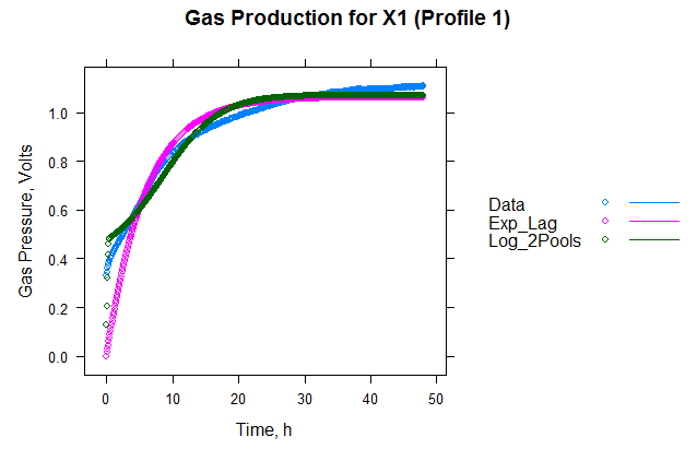
Gas production plots of alfalfa hay generated with the GasFit System 4.x |
|
|

Download
|
It uses R! |
Visual Studio 2026 |
|
32 bit and 64 bit Compatible |
|
The GasFit System software is programmed with Microsoft Visual Studio using Visual Basic and the .NET Framework 4.8.1 (click here to download the .NET Framework). It uses R scripting v. 4.x or later technology (Click here to download R) to perform calculations, nonlinear convergence, and high-quality graphic production. It works with most IBM-PC compatible computers that have Microsoft Windows 10 or later. In order to execute GasFit System, you have to install the following R packages: XML, lattice, chron, minpack.lm, and ggplot2. Version 4 added minpack.lm (Levenberg-Marquardt convergence) and ggplot2 (all of the charts), so a computer that ran an earlier version will need those two. Even though GasFit System will try to install them automatically, you may install them manually. Briefly, after you have installed R, open R, click on menu packages, and then install packages. Select the provider and then select the package one at a time. You have to have an internet connection active to download the packages. There is a Visual Basic Script (Install R Packages.VBS) in the GasFit System folder that performs the installation of these packages automatically. |
|||



The current version of the GasFit System is Loading...

What is new in GasFit System version 4? NEW
- An HTML report of every run. A single report.html page is written into the results folder and can be opened automatically when the run finishes. It carries a run summary, one card per profile with the selected model, its formula and fitted parameters, every model ranked by residual sum of squares with ΔAIC and a converged / failed / switched-off badge, the polynomial reference fits, and all of the charts.
- Every chart redrawn. The all-models comparison is now one small panel per model, ordered best fit first, so the curves no longer overlap in a single band; the model-error chart is sorted relative to the best model and switches to a logarithmic axis when the spread is wide; the raw-data chart carries a local smooth with a 95% confidence band; and the chart files are named so that the results folder sorts into reading order.
- Two new spreadsheet-friendly result files. Model Fit Statistics.csv gives one row per profile and model, with model names and converged / selected flags, and Fitted Values.csv gives time, profile, model, predicted value, and residual in a single tidy table. The original result files are unchanged, so existing spreadsheets keep working.
- Levenberg-Marquardt convergence is available and is now the default fitting algorithm, alongside Gauss-Newton, port, and plinear.
- Considerably faster. The fixed cost paid at the start of every run was cut by about two-thirds, and the fitting itself is faster; the Richards model in particular is roughly forty times quicker.
- Corrected statistics and a corrected model. The reported sum of squares, coefficient of determination, iteration counts, and the two-pool models were all fixed. Please see the Support section for the full list.
At Texas A&M University (TAMU), we have created some templates to assist in preparing gas production data to be evaluated with the GasFit System. Our gas production system uses Pico Technology (PICOTECH) software. The following templates are provided without any support, some adjustments might be needed depending on the gas production system used.
- Previous versions can be downloaded from here.
- A list of modifications can be found here.
- The latest Gasfit templates are:
- GasFit Template v. 43 for the Texas A&M University system
- Ankom 2009 Template for the ANKOM system
- The latest script for GasFit is:
- GasFit script 4.2.0
- Unzip the zip file and copy the .ZZZ file to the My Documents\NutritionModels\GasFit Files\Scripts folder

A tutorial on how to install and use the GasFit System is available at the Media web page.
Registration
The GasFit System will expire after 10 trial uses if it is not registered by the end of the grace period. You may register your copy by submitting the license number on the Register webpage. If applicable, registration codes are issued only after the full registration fee has been paid on the Purchase webpage.
Developers

|
Dr. Luis O. Tedeschi
|

|
Support
The following list summarizes corrections, enhancements, and functional improvements made to the software, presented in chronological order (newest to oldest). Each entry reflects updates implemented to improve stability, usability, and overall performance. GasFit has two parts that are released together and are versioned separately: the Windows program, which prepares the run and displays the results, and the R script, which performs all of the fitting, statistics, and graphics. They are listed below under their own headings.
August 2026. In the update v. 4.0.9737.21556, the spelling was standardized throughout to American English in the GasFit program and R script. In the update v. 4.0.9736.33246, the third-party interface controls and the shared registration and webupdate libraries were brought up to their current releases, and GasFit was rebuilt against them. This is internal maintenance with no effect on how GasFit is used — the program, the fitting script and the results it produces are unchanged from the previous version 4.0 release. It keeps the program current with the components it depends on, and it is the reason a new build was issued.
GasFit v. 4.0 (changes since v. 3.x)
- Corrected. The main window could freeze during a run. Once the R script had produced more than a few kilobytes of output the program stopped responding, and it never recovered; stopping a run part-way through froze it as well. The run is now driven by events and the output is read as it is produced, so a long run keeps the progress window updating and the Stop button working.
- Corrected. Projects saved with Levenberg-Marquardt came back with no fitting method. Neither the Levenberg-Marquardt selection nor the plot resolution was written to the project file, and because the file did record the other three methods as unselected, reloading such a project left the whole group blank and the run was started without a fitting method at all. Both settings are now saved, and older project files continue to load unchanged.
- Added. Open report. A new option on the main window opens the run's HTML report (see the R script section below) as soon as the run finishes.
- Improved. Failures are now named. A crash inside one of the R packages, or an unhandled error in the script, used to end the run with an unexplained negative number. Both now report a described result, and the reason is written to the log and to the captured output.
- Corrected. Several smaller defects: (1) a leading space in the initial or final profile box stopped the run with a conversion error before R was even launched; (2) where more than one version of R is installed the newest is now preselected correctly, as version 4.10 was previously treated as older than version 4.9, and duplicated entries in the list were removed; (3) opening the About window consumed one of the trial uses; (4) every script load left a temporary file behind; (5) the update notice could appear behind the splash screen and stall start-up; (6) the splash screen was rebuilt and no longer clips its text on high-resolution displays; and (7) the update and registration settings, which had been duplicated in two places and had drifted apart, are now held in one place each.
GasFit R Script v. 4.0 (changes since v. 3.x)
- Corrected. A run could terminate outright, with no message. One of the GnG1 model functions returned nothing at all outside the region it was written for, which ended the whole process part-way through the first profile with no error and no results. The same hole was corrupting the parameter grid search, because that empty result scored as a perfect fit and therefore won the search. Model functions now return a valid, penalized value over the entire parameter range.
- Corrected. The wrong sum of squares was reported in five places. The regression sum of squares was being used and labeled as the error sum of squares in the per-profile error chart, the model comparison table printed into each profile file, the across-profile error chart, the summary statistics file, and the model distribution charts. Because the regression sum of squares is dominated by the total sum of squares, the models came out nearly identical and the error charts ranked them in reverse order. All five now use the error sum of squares, which is also the quantity the best model is selected on.
- Corrected. The GnG1 models reported one minus the coefficient of determination in place of the coefficient of determination, and an adjusted value derived from it. The other models were unaffected.
- Corrected. The two-pool GnG1 model had never converged for any profile. A pool with n equal to one contains no lag parameter, so fitting one made the problem singular at every starting value. That parameter is no longer fitted where it does not exist: the two-pool form now converges for every profile, and the one-pool case with n equal to one, which is the exponential model, is skipped with the reason given in the log.
- Corrected. Creating a new parameter file could overwrite the wrong file, and produced an unusable one. The new file was written to the working folder instead of to the file named on the main window, so the program could warn about one file and replace another. The grid steps it generated were also far finer than the shipped values, which multiply together across a grid; one model required roughly eight gigabytes of memory. The generated file now matches the shipped working values.
- Added. An HTML report of every run. A single report.html page is written into the results folder at the end of every run. It carries a run summary, one card per profile with the selected model, its formula and fitted parameters, every model ranked by error sum of squares with ΔAIC and a converged / failed / switched-off badge, the polynomial reference fits, and all of the charts.
- Added. Results are organized into folders. A thirty-profile run writes more than two hundred files, and previously all of them landed in one directory where the charts buried the tables. The charts are now in plots, the spreadsheets in csv, and the text output in text, with the log, the report, and the results table at the top level.
- Added. Two spreadsheet-friendly result files. Model Fit Statistics.csv gives one row per profile and model, with model names and converged / selected flags, and Fitted Values.csv gives time, profile, model, predicted value, and residual in a single tidy table, instead of one column per model and profile pair. The original result files are unchanged, so existing spreadsheets keep working.
- Improved. Every chart was redrawn on the ggplot2 graphics package under a single theme. The all-models chart is now one small panel per model, ordered best fit first, instead of overlapping curves drawn in six repeated colors; the model-error chart is scaled relative to the best model rather than the worst, and switches to a logarithmic axis when the spread is wide; the best-fit and polynomial charts no longer draw a dense profile as one solid mass; and the raw-data chart carries a local smooth with a 95% confidence band. Chart file names now begin with a number so the folder sorts into reading order.
- Improved. Levenberg-Marquardt is available and is now the default fitting algorithm, alongside Gauss-Newton, port, and plinear.
- Improved. Considerably faster. The fourteen named models are now driven by a single description table rather than fourteen repeated blocks of script, which cut the fixed cost paid before the first profile is fitted from about thirteen seconds to about four. A successful search is no longer followed by an identical second fit, and the Richards model, which had been starting from a value outside its own valid range and therefore falling back to an exhaustive grid search on every profile, is roughly forty times quicker. The fitted values themselves are unchanged.
- Improved. Several smaller corrections: (1) the Iterations column of the result files was always empty and is now recorded for every model and profile; (2) the Gompertz with intercept model was scoring its parameter grid with another model's objective function, so its starting values were effectively chosen at random; (3) the Cone model's own grid step was read from the parameter file and then ignored; (4) one grid lower bound was set to a value at which the model is constant in time; (5) chart label sizes no longer change when the plot size is changed; and (6) Summary Table.csv gained the selected model's name, which had been only a number.
Several related documents, manuscripts, and reports are listed on the Publications web page, such as:
- Tedeschi, L.O., Schofield, P., Pell, A.N., 2008. Determining feed quality for ruminants using in vitro gas production technique. 1. Building an anaerobic fermentation chamber. In: Arcuri, P. B. (Ed.) The 4th Workshop on Modeling in Ruminant Nutrition: Application of the Gas Production Technique. EMBRAPA, Juiz de Fora, MG, Brazil, p. 16 p.
- Tedeschi, L.O., Schofield, P., Pell, A.N., 2008. Determining feed quality for ruminants using in vitro gas production technique. 2. Evaluating different models to assess gas production measurements. In: Arcuri, P. B. (Ed.) The 4th Workshop on Modeling in Ruminant Nutrition: Application of the Gas Production Technique. EMBRAPA, Juiz de Fora, MG, Brazil, p. 15 p.
Links
This section will be updated with relevant links as they are identified and curated for this model.